
Cosmic string dynamics and evolution
How do cosmic strings evolve?
The evolution of cosmic string network is the relatively complicated result of only three rather simple and fundamental processes: cosmological expansion, intercommuting & loop production, and radiation. We describe each one of them below...
Cosmological expansion
The overall expansion of the Universe will 'stretch' the strings, just like any other object that is not gravitationally bound. You can easily understand this through the well-known analogy of the expanding balloon. If you draw a line of the surface of the balloon and then blow it up, you will see that the length of your 'string' will grow at the same rate as the radius of the balloon.
The processes of intercommuting and loop production
Intercommuting & loop production
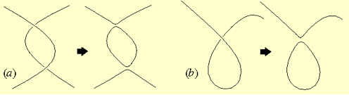
Whenever two long strings cross each other, they exchange ends, or 'intercommute' (case (a) in the figure on the right). We had already encountered this apparently strange fact when we discussed the strings in the context of nematic liquid crystals. In particular, a long string can intercommute with itself, in which case a loop will be produced (this is case (b) in the figure on the right).
Below you can see two movies providing numerical evidence for the intercommuting process. Figure 1 shows a full three-dimensional simulation of the intercommuting of two cosmic strings, while Figure 2 shows a two-dimensional section of it. The height of the surface above the plane represents the energy present at each point.
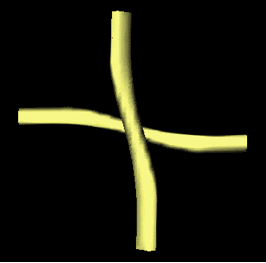
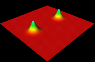
Figure 1. (left) The reconnection and 'exchange of partners' when two strings intersect. In this three-dimensional simulation, the strings approach each other at half the speed of light. Notice the radiation of energy and the production of a small interaction loop in the aftermath of the collision (R. Battye & E.P. Shellard)
Figure 2. (right) The scattering of two vortices is highly non-trivial; the two vortices approach and form a donut from which they emerge and right-angles and have 'exchanged halves' (J. Moore & E.P. Shellard)
Radiation
Both long cosmic strings and small loops will emit radiation. In most cosmological scenarios this will be gravitational radiation, but electromagnetic radiation or axions (an as yet undiscovered but hypothesised elementary particle can also be emitted in some cases (for some specific phase transitions). Figure 1 below presents a single, oscillating piece of string and Figure 2 shows the radiation that is being emitted. Note that this is a cross section through the string, that is, in this movie the string is perpendicular to the screen.
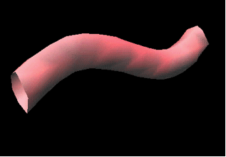
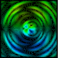
Figure 1. (left) Three-dimensional simulation of an oscillating cosmic string (actually a global string). The motion of the string which is held at either end is periodic, but the amplitude slowly decays because of radiation as shown below (R. Battye & E.P. Shellard)
Figure 2. (right) Radiation fields from the oscillating shown above. A transverse cross-section of the fields has been made at the point of maximum amplitude. Notice the four lobes of the radiation (a quadrupole pattern) which is characteristic of all cosmic string radiation (R. Battye & E.P. Shellard)
The effect of radiation is much more dramatic for loops, since they lose all their energy this way, and eventually disappear. Here you can see what happens in the case of two interlocked loops. This configuration is unlikely to happen in a cosmological setting, but it is nevertheless quite enlightening. Notice the succession of complicated dynamic processes before the loop finally disappears!
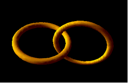
If you are not able to see the movie, here are some selected snapshots...
So, what's the overall effect?
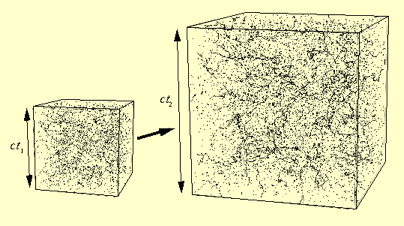
Scale-invariant evolution of a cosmic string network. The network looks exactly the same (in a statistical sense) if it is re-scaled relative to the horizon (which grows in proportion to the time, t, multiplied by the speed of light, c)
After formation, an initially high density string network begins to chop itself up by producing small loops. These loops oscillate rapidly (relativistically) and decay away into gravitational waves. The net result is that the strings become more and more dilute with time as the Universe expands. From an enormous density at formation, mathematical modelling suggests that today there would only be about 10 long strings stretching across the observed Universe, together with about a thousand small loops!
In fact the network dynamics is such that the string density will eventually stabilize at an exactly constant level relative to the rest of the radiation and matter energy density in the Universe. Thus the string evolution is described as 'scaling' or scale-invariant, that is, the properties of the network look the same at any particular time t if they are scaled (or multiplied) by the change in the time. This is schematically represented on the right.
In order to obtain a more detailed description of the evolution, however, it is necessary to use high-resolution numerical simulations.