
High-resolution cosmic string simulations
Why do we need numerical simulations?
Because strings are extremely complex non-linear objects. The only rigorous way to study their evolution and cosmological consequences is to create numerical simulations on the computer. These, however, are very difficult to perform, and in order to be accurate enough they require extremely long CPU times, even in computers as powerful as COSMOS. Indeed, there are only two research groups in the world which have accurate string codes!
Therefore, one of the aims of performing numerical simulations of the evolution of cosmic string networks is to subsequently use the resulting information as an input to build (relatively) simpler analytic models that reproduce (in an averaged sense) the crucial properties of these objects.
What does the string code do?
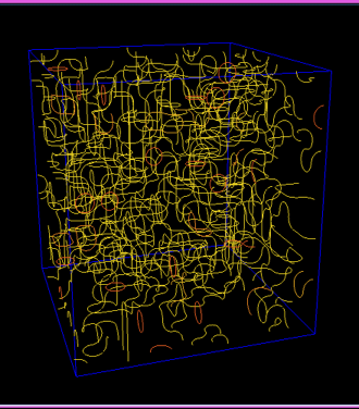
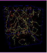
A snapshot of a typical initial string box. Notice that the displayed box is only a fraction of the total simulation box (C. Martins & E.P. Shellard)
The code we use was originally developed by Bruce Allen and Paul Shellard, and has recently been upgraded. It has over 20000 lines of C code. It starts by generating an initial 'box of strings' (see below), containing a configuration of strings such as one would expect to find after a phase transition in the early Universe. Then it evolves this initial box, by using the laws of motion of the strings to determine how it should look like a bit later (such an interval is called a 'timestep').
Notice that in this and all other pictures and movies below long strings are shown in yellow, while small loops have a colour code going from yellow to red according to their size (red loops being the smallest).
This is then repeated for a very large number of timesteps. The code then outputs information about the configuration of strings in the box at each timestep. Additional code and standard software tools are then used to convert this into a 'frame'. Finally, all the frames are put together in a movie. We have one frame per timestep, but in the movies shown below only one of every 10 is used.
At each timestep the code can also calculate and output a very large number of relevant statistical properties of the network. These are then put through additional data analysis software, in order to extract information that is relevant for the subsequent process of analytic model building.
The code is prepared to run in a number of different cosmological scenarios. For example, one expects the properties of the string networks to be quantitatively different at very early times when the Universe was dominated by radiation and relativistic particles (this is known as the radiation era) or at later times, when it became dominate by non-relativistic particles (this is known as the matter era)

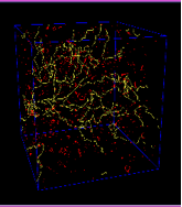
Snapshot of a string network in the radiation era (click for a larger view). Note the high density of small loops and the 'wiggliness' of the long strings in the network. The box size is about 2ct (B. Allen & E.P. Shellard)

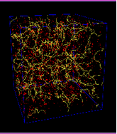
Snapshot of a string network in the matter era (click for a larger view). Compare with the radiation case. Notice the lower density of both long strings and loops, as well as the lower 'wiggliness' of the former. The box size is again about 2ct (B. Allen & E.P. Shellard)
It is possible to simulate both of these regimes, as well as the transition between them. We will explain the differences between them below. We can also perform simulations with or without the expansion of the Universe, in order to learn what its effect is on the properties of the strings.
Why do the two boxes look different?
Because the rate at which the Universe is expanding is different. At very early times the energy density of the Universe is dominated by radiation (and relativistic matter). In this case the Universe expands relatively slowly. On the other hand, in the later stages, non-relativistic (slowly-moving) matter dominates the Universe. In this case the expansion is relatively fast. This transition between the two different epochs happens between 1,000 and 10,000 years after the Big Bang.
The change in this rate of expansion does not affect the qualitative 'scaling' evolution of a string network that we described previously. However, it does change the detailed properties of the network. In order to maintain scaling, a network needs to be diluted at a sufficient rate, and this is done by the three effects we discussed previously: expansion, intercommutation and radiation.
In the radiation era the Universe expands relatively slowly and the string network is not stretched a great deal. In order to be diluted at a sufficient rate to maintain 'scaling', the network must chop off a large number of small loops. The poor string stretching and the extra reconnections required to form loops also result the strings becoming 'wiggly' that is, the strings possess a large amount of small-scale structures. This has important consequences for string dynamics. A detailed description of these effects is important if we are to make quantitative predictions about the cosmological implications of cosmic strings.
In the matter era, the expansion rate is comparatively faster. The string network is, therefore, considerably stretched, so it is already 'half-way' to maintaining 'scaling'. Thus a much smaller loop production rate is required, and this with its correlation length also growing. The remainder of the dilution required is achieved through the formation of small loops (coloured red in the pictures). Understanding string evolution during the matter epoch from a few thousand years through to the present day is important for predicting their potential role in galaxy formation.
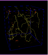
Here you can see a series of snapshots from a cosmic string network that is evolving during the transition from the radiation epoch to the matter epoch. Notice the gradual changes in the string density and the number of loops! Click on each image to see a larger version of it!
How long does the code run for?
In the past 15 months, we have performed about 90000 CPU hours of cosmic string network evolution runs on the COSMOS supercomputer. This is about 10 years of real time! A single run typically contains around ten million points and runs for about 10 weeks of real time using 8 processors.
Each run can have up to ten thousand timesteps, and at each one of them the code outputs up to about 100Mb of 'useful' data. this does not include other files that are used for checkpointing. These are the largest and most accurate cosmic string simulations performed to date.
And now for the movies!
Below you can find movies of the evolution of cosmic string networks in both the radiation and matter eras. For each of the two cosmological epochs, there are two movies. In the first one, the displayed box has a fixed size, so as the movie proceeds you will see progressively less strings. This is due to the fact that the Universe is expanding, whereas the box is not.
On the other hand, in the second one the box expands with the comoving horizon. In this case you will see the strings progressively 'falling into' the box. Nevertheless, you should notice that the number of long strings in the box remains roughly constant, in agreement with the scaling hypothesis. This is because the additional length in strings is quickly converted into small loops.
You should also notice the differences in the network properties in the radiation and matter eras, as discussed above.
Two movies of the evolution of a cosmic string network in the radiation era. In the movie on the left, the box has a fixed size, while in the one on the right it grows with the comoving horizon (C. Martins & E.P. Shellard)
Why are the simulations useful?
Although the movies are in some sense a nice by-product of the simulation, they can provide extremely useful insights into the detailed dynamics of the strings. For example, if you look carefully you will notice that the formation of loops is actually a two-stage process. First, a long string produces a relatively large 'mother-loop', and then this loop decays into a number of much smaller 'daughter-loops'. This can be seen through careful analysis of the time evolution of the statistical properties of the network, but it becomes obvious when one sees a movie of it. Question: Can you estimate how many 'daughter-loops' are typically produced by each 'mother-loop'?
Two movies of the evolution of a cosmic string network in the matter era. In the movie on the left, the box has a fixed size, while in the one of the right it grows with the comoving horizon (C. Martins & E.P. Shellard)
When one wants to build an analytic model for cosmic string evolution, the main goal is to be able to predict how a number of averaged properties of the network evolve in time. Simple examples of such properties are the number of long strings in a given volume, the average string velocity, the typical distance between two long strings, and the number and size of the loops produced by the long strings. Slightly less obvious ones are the correlation length (the typical distance over which a long string is roughly straight, before bending into a different direction), as well as quantities measuring the amount of 'wiggles' that each string has.
Obviously, all this information can be extracted (after some additional data processing work) from a simulation. In this way, one can test for the accuracy of one's favourite analytic model, and obtain valuable clues about how successful modelling should proceed.
Once one is confident that an adequate analytic model of string evolution is available, one can use it as a powerful tool to analyse the detailed cosmological consequences of cosmic strings.